class: center, middle, inverse, title-slide # Estimating Berlin House Prices using rstanarm ### <br>Corrie Bartelheimer <br /> <br /> <br> ### June 15, 2019 --- # The Data -- <!-- --> --- ## What are good predictors? -- - Size -- - Location, location, location --- ## How to include ZIP codes in your model? -- - Encoding, e.g. One-Hot-Encoding -- - Categorical embedding -- - One model per ZIP code -- - Omit -- - **Hierarchical model** --- ## Hierarchical Model In short: A compromise between **one model per ZIP code** (no pooling) and **ignoring ZIP code information** (complete pooling). A hierarchical model does **partial pooling** --- ## The model .large[ `$$\begin{align*} \text{Price} &\sim \text{Normal}(\mu, \sigma) \\ \\ \\ \mu &= \alpha_{[ZIP]} + \beta_{[ZIP]} \text{area} \\ \\ \\ \begin{bmatrix}\alpha_{[ZIP]} \\ \beta_{[ZIP]} \end{bmatrix} &\sim \text{Normal}( \begin{bmatrix} \mu_{\alpha} \\ \mu_{\beta} \end{bmatrix}, \Sigma) \end{align*}$$` ] --- ## How to compute it -- > RStanArm allows users to specify models via the customary R commands, where models are specified with formula syntax. -- ```r library(rstanarm) options(mc.cores = parallel::detectCores()) mod <- stan_lmer( price.s ~ area.s + (1 + area.s | plz) , data=df.model) ``` -- A simpler model for comparison: ```r mod_simple <- stan_glm( price.s ~ area.s , data=df.model) ``` `price.s` is the price in 100,000€s, `area.s` is the standardized living area. --- ## What about priors? Wikipedia: > A prior, [..] is the probability distribution that would express one's beliefs about this quantity before some evidence is taken into account. Or: **How much do we know about the problem before seeing the data?** --- ## What about priors? RStanArm uses by default **weakly regularized** priors -- ```r prior_summary(mod) ``` ``` Priors for model 'mod' ------ Intercept (after predictors centered) ~ normal(location = 0, scale = 10) **adjusted scale = 21.58 Coefficients ~ normal(location = 0, scale = 2.5) **adjusted scale = 5.40 Auxiliary (sigma) ~ exponential(rate = 1) **adjusted scale = 2.16 (adjusted rate = 1/adjusted scale) Covariance ~ decov(reg. = 1, conc. = 1, shape = 1, scale = 1) ------ See help('prior_summary.stanreg') for more details ``` --- ## What about priors? Visualize the priors: ```r default_prior <- stan_glm( price.s ~ area.s, * prior_PD = TRUE, data=df.model) ``` -- .center[ 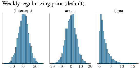 ] --- ## What about priors? .center[ 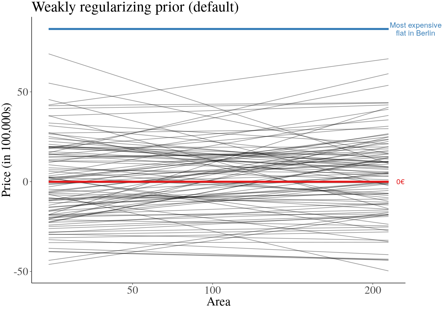 ] --- ## What about priors? We can of course also fit our own priors: ```r mod <- stan_lmer( price.s ~ area.s + (1 + area.s | plz) , data=df.model, prior_intercept=normal(location=3, scale=2.5, autoscale = FALSE), prior=normal(location=1, scale=1, autoscale=FALSE)) ``` -- .center[ 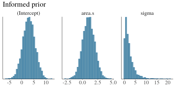 ] --- ## What about priors? .center[ 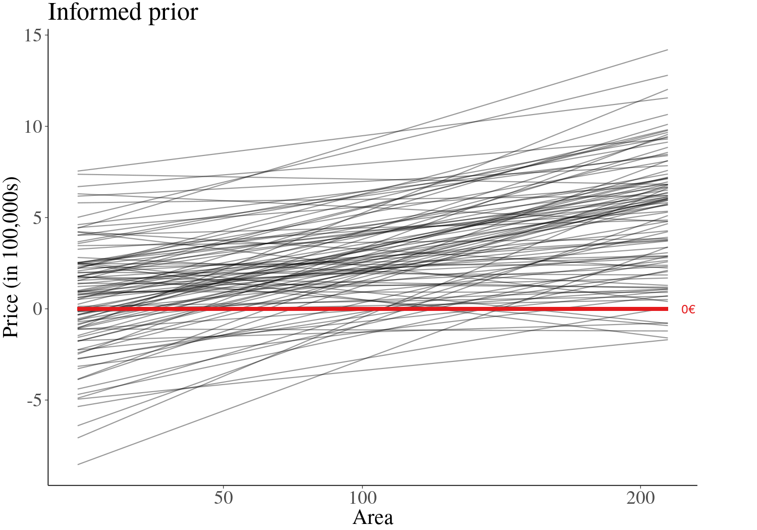 ] --- ## Assessing convergence ```r launch_shinystan(mod) ``` --- class: center, middle .gif[  ] --- ## Model comparison -- ```r library(loo) l_mod <- loo(mod) l_simple <- loo(mod_simple) compare_models(l_mod, l_simple) ``` ``` Model comparison: (negative 'elpd_diff' favors 1st model, positive favors 2nd) elpd_diff se -1903.6 135.5 ``` --- ## Analyzing the results & Prediction -- Extract fitted draws ```r mitte <- c("10119", "10178", "10179", "10783") library(tidybayes) library(modelr) df.model %>% filter(plz %in% mitte) %>% group_by(plz) %>% * data_grid(area.s = seq_range(area.s, n=100)) %>% * add_fitted_draws(mod, n=50) %>% head() ``` ``` # A tibble: 6 x 7 # Groups: plz, area.s, .row [1] plz area.s .row .chain .iteration .draw .value <chr> <dbl> <int> <int> <int> <int> <dbl> 1 10119 -1.16 1 NA NA 12 1.26 2 10119 -1.16 1 NA NA 53 2.00 3 10119 -1.16 1 NA NA 66 1.48 4 10119 -1.16 1 NA NA 301 1.94 5 10119 -1.16 1 NA NA 380 1.25 6 10119 -1.16 1 NA NA 530 1.18 ``` --- ## Analyzing the results & Prediction .center[ 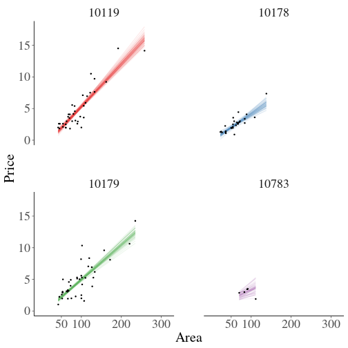 ] --- ## Analyzing the results & Prediction Extract posterior predictions ```r df.model %>% filter(plz %in% mitte) %>% group_by(plz) %>% data_grid(area.s = seq_range(area.s, n=100) ) %>% * add_predicted_draws(mod, n=100) %>% head() ``` ``` # A tibble: 6 x 7 # Groups: plz, area.s, .row [1] plz area.s .row .chain .iteration .draw .prediction <chr> <dbl> <int> <int> <int> <int> <dbl> 1 10119 -1.16 1 NA NA 1 2.15 2 10119 -1.16 1 NA NA 2 0.221 3 10119 -1.16 1 NA NA 3 -0.421 4 10119 -1.16 1 NA NA 4 1.68 5 10119 -1.16 1 NA NA 5 2.28 6 10119 -1.16 1 NA NA 6 2.23 ``` --- ## Analyzing the results & Prediction .center[ 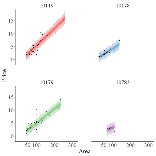 ] --- ## Analyzing the results & Prediction We can predict using the RstanArm function `posterior_predict()` ```r nd <- data.frame(area.s=standardize(101), plz="10407") post <- posterior_predict(mod, newdata=nd) ``` .center[ 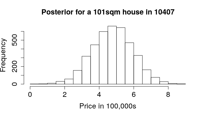 ] --- ## What is the probability We can use the posterior to answer questions such as > "What is the probability that a house in 10407 (Prenzlauer Berg) of 101sqm has a price less than 300,000€?" ```r mean( post < 3 ) ``` ``` [1] 0.065 ``` -- .center[  ] --- ## Visualizing the Results Price estimate for an average house (104sqm) .center[  ] --- Slope - Estimate for the price per sqm .center[  ] --- Posterior Probability that a house of 101sqm has a price less than 300,000€ .center[  ] --- ### Closer look on 12047 .center[  ] --- ## Things to improve -- - Many outliers in the data -- - Price for large houses difficult to predict -- - Important predictors still missing -- - Object type (e.g. house or flat) -- - Time -- - No information about similarity of neighborhoods included -- - Multiple Levels --- ## Summary - Houses in Berlin are expensive -- - Affordable locations are mostly outside the ring -- - RStanArm and co make Bayesian modelling very accessible -- - For more complex models, use RStan or brms --- ## Thank you! - Questions? - Slides and Code on <i class="fab fa-github "></i>: [https://github.com/corriebar/Estimating-Houseprices](https://github.com/corriebar/Estimating-Houseprices) - <i class="fab fa-twitter "></i> [@corrieaar](https://twitter.com/corrieaar) - Blog: [https://www.samples-of-thoughts.com/](https://www.samples-of-thoughts.com/) - <i class="fab fa-meetup "></i> If want to learn more, come to our meetup: [http://meetu.ps/c/41dg1/v14wk/f](http://meetu.ps/c/41dg1/v14wk/f) .center[ <img src="images/meetup.jpeg" height="130" /> ]